C++ is a great programming language to calculate engineering problems, it is one of the best for those operations. Delphi is also faster compiled programming language that you can use in engineering problems. In this post we will explain how to write a C++ app to solve millions of unknowns in Equations by using Successive Over Relaxation Iteration Method.
Table of Contents
A little about the mathematics behind this C++ app
In mathematics there are Implicit Equations and we Engineers mostly faced on solving numerical equations about the real-life problems. Thermodynamics, Fluid Mechanics, Mechanism Theories, Structure Analysis, and many other engineering areas requires to solve many unknown equations. Sometimes calculations these should be in real time, or it should be simulating time fractions very precisely. Generally, these implicit equations are exposed on a 1D, 2D or 3D grid examples (i.e compressed on uncompressed fluid flow, thermal distributions) and these grids has nodes with parameters (i.e. Velocity, Pressure, Temperature etc.)
In mathematics, an implicit equation is a relation of the form R(x1,…, xn) = 0, where R is a function of several variables. In example, the implicit equation of the unit circle is is x2 + y2 − 1 = 0. More complex equations can be given as equations about to solve first and second law of thermodynamics, Momentum Equations, Naiver-Stokes Equations etc.
An Implicit Function is a function that is defined by an implicit equation, that relates one of the variables, considered as the valueof the function, with the others considered as the arguments. These Implicit Equations can be solved by using iteration methods.
How to solve a 3-diagonal matrix in C++
One of the most popular methods is SOR Successive Over Relaxation Iteration Method (SOR). This method can be used to solve problems on 1D, 2D and 3D problems. In Numerical Linear Algebra, the Successive Over-Relaxation (SOR) Method is a variant of the Gauss–Seidel method for solving a linear system equation, resulting in faster convergence. A similar method can be used for any slowly converging iterative processes.
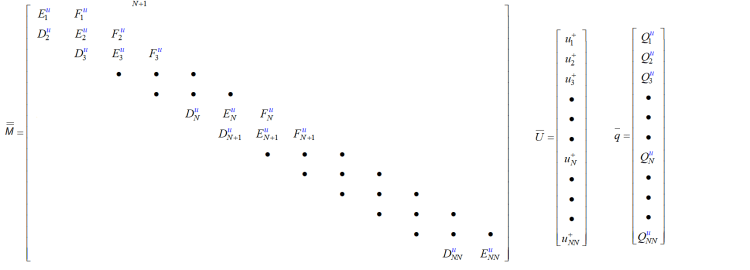
Implicit Equations on 1D Grids produces Triangular Matrix forms. If the problem is on a 1D grid (for example heat transfer on a wire is 1D problem) this will produce 3 diagonal matrix forms. Because each 1D grid nodes on this wire connected to with left node and right except the first and the last one. That means there will be 3 variables (Left, Mid, Right) in each lines of the 2D matrix affecting to 3 Unknowns that we want to solve.
Simply equations in matrix form can be written as below.

In this equation;
M is 2D matrix (2 bars shows that it is 2D matrix),
U is 1D matrix form of unknown parameters from the each node,
q is 1D matrix form of right side of the equation.
These M, U and q matrixes can be shown as below here,

Here is C++ app example of how to solve a 3-diagonal matrix
|
1 2 3 4 5 6 7 8 9 10 11 12 13 14 15 16 17 18 19 20 21 22 23 |
//--------------------------------------------------------------------------- #include <vcl.h> #pragma hdrstop #include "SOR_Iteration_Unit1.h" //--------------------------------------------------------------------------- #pragma package(smart_init) #pragma resource "*.dfm" #define max(__a,__b) (((__a) > (__b)) ? (__a) : (__b)) #define min(__a,__b) (((__a) < (__b)) ? (__a) : (__b)) #define NN 10 // Number of Nodes TForm1 *Form1; double m[NN+1][NN+1], u[NN+1], x[NN+1], sol[NN+1]; //--------------------------------------------------------------------------- __fastcall TForm1::TForm1(TComponent* Owner) : TForm(Owner) { } |
If you don’t have any equation or example matrix, we can generate random 3 diagonal equations to test as given below,
|
1 2 3 4 5 6 7 8 9 10 11 12 13 14 15 16 17 18 19 20 21 22 23 24 25 26 27 28 |
void generate_random_3diag_equations() { int i,j; srand( time(0)); for(i=0; i<NN; i++) u[i]=i; // First Line, Top Left Corner m[0][0] = (1+rand()%100)/100.0; // central node m[1][0] = (1+rand()%100)/100.0; // right node x[0] = u[0]*m[0][0] + u[1]*m[1][0]; // u0*E + u1*F for(j=1; j<NN-1; j++) { m[j-1][j] = (rand()%100+1)/100.0; // left node m[ j ][j] = (rand()%100+1)/100.0; // central node m[j+1][j] = (rand()%100+1)/100.0; // right node x[j] = u[j-1]*m[j-1][j]+ u[j]*m[j][j]+u[j+1]*m[j+1][j]; } // Last Line, Bottom Right Corner j = NN-1; m[j-1][j] = (rand()%100+1)/100.0; // left node m[j][j] = (rand()%100+1)/100.0; // central node x[j] = u[j-1]*m[j-1][j]+ u[j]*m[j][j]; } |
Solving a linear equation in a C++ app
Linear equations can be solved by Successive Over Relaxation (SOR) Method. Here we developed a SOR Revised Method (SORR) in C++ as below,
|
1 2 3 4 5 6 7 8 9 10 11 12 13 14 15 16 17 18 19 20 21 22 23 24 25 26 27 28 29 30 31 32 33 34 35 36 37 38 39 |
unsigned int calc_SOR( const unsigned int max_iteration ) { const double omega = 0.5; const double min_error = 0.0001; double err; double prev, next, psol; unsigned int iteration =0; do { err=0; for(int j=0; j<NN; j++) { prev=0; next=0; for(int i=0; i<j; i++) prev += m[i][j] * sol[i]; // these lines costly for(int i=j+1; i<NN; i++) next += m[i][j] * sol[i]; // these lines costly psol = sol[j]; sol[j]=(1.0-omega)*u[j] + omega*(x[j]-prev-next)/m[j][j]; err += pow( sol[j]-psol, 2); } err = err/NN; // this line can be removed for(int i=0; i<NN; i++) u[i]=sol[i]; iteration++; Form1->Memo1->Lines->Add( UIntToStr(iteration) + ":" +FloatToStrF( err, TFloatFormat::ffFixed, 12, 6 ) ); }while(min_error<err && iteration<max_iteration); return iteration; } |
For example, we can calculate unknowns with maximum 1000 iterations by using this calc_SOR() function as below,
|
1 |
void calc_matrix_SOR(1000); |
C++ is a great programming language to solve these kind of equations.
Design. Code. Compile. Deploy.
Start Free Trial
Free C++Builder Community Edition

